Asteroids
Menekay, Deniz - Mert Ünsal, Fahri - Kempen, Friedrich - You, Tianyi
In this semester, group 1 of the Astronomy club worked on tracing asteroids, especially Gertrud and Arkhipova. We tracked and took pictures of the two asteroids to the extent permitted by the weather and dome’s hydraulic system, then derived their orbits with the help of Astrometrica.
1. Photographing Asteroids
The first step was finding which asteroid to photograph. The rule of thumb is that the IAPG telescope is able to observe objects in the sky up to 17.0 apparent magnitude. Considering that, we listed asteroids we can observe in Munich with the help of the Minor Planet Checker of the Minor Planet Center (MPC) [1].
Since it was our first time observing asteroids, we chose (710) Gertrud and (4424) Arkhipova to be on the safe side. The reason was that these two asteroids were observed a short time
ago in the observatory. From Munich, Gertrud was a relatively bright asteroid with an apparent magnitude of ∼15 throughout the observation period. Arkhipova was dimmer with an apparent magnitude of ∼16 in the same time period.
First observations were done by tracking the asteroid through KStars, which controls the mount. The telescope was pointed to the target asteroid and 3-5 pictures were taken at intervals of ∼10 minutes. We used an exposure of 150 seconds. It has been tested to be a good value to observe asteroids in the 14 to 17 magnitude range, with the current setup at the IAPG Observatory. This was done by obtaining the current right ascension and declination through Stellarium, then entering values to the mount manually. KStars software was used to control the camera and obtain pictures. Keep in mind that photos taken this way do not contain RA and Declination values in metadata. We took note of it and manually enter Astrometrica in the “Data Reduction” part. RA and Dec values were defined based on the latest star catalog in Astronometry.net.
2. Processing Images via Astrometrica
After obtaining pictures, the next step was to upload them to Astrometrica software and process images. Astrometrica is a tool for data reduction of CCD images, which is specially designed for minor bodies of the solar system such as asteroids, comets, and dwarf planets [2]. Automatic image calibration, data reduction, image blinking, and automatic moving object detection functions are what make Astrometrica ideal for discovering and taking follow-up-observation of asteroids.
Some of the settings must be changed once you download the software and open it for the first time. Both the location of the observatory and the specification of the gear in use should be changed in the settings. Additionally, it is recommended to use the Gaia DR2 star catalog with Quadratic Fit.
After uploading images to the software with the .fits extension, the following step was to make “Astrometric Data Reduction”. In case RA and Dec were not saved in the picture metadata, they are entered manually in Astrometrica. This happened to be the case when we had to control the mount manually. The command extracts stars from the image and
automatically matches them with the star catalogue. In case the software could not succeed, you can match stars manually. The second step was running “Known Object Overlay”, which displays the position of minor planets according to the MPC Orbit databases. So that we can have a rough idea about where asteroids are on the image.
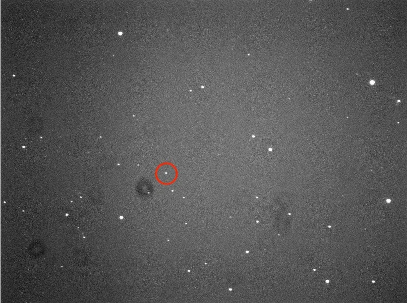
Asteroids have a different motion path than stars. Thus, “Blink Current Images” function helps you to find the asteroid in the image. If the asteroid is already known by the MPC database, it is likely that the asteroid you are looking for will be close to the defined location from the “Known Object Overlay”. Inverting the image colors can help you to find the object easier.
After finding and assigning asteroids, it is seen that there is a deviation of RA and Declination between our observation and MPC database as follows:
| Date of Observation | Asteroid | dRA [arcminute] | dDe [arcminute] |
| 22.03.2022 | Gertrud | -1.0 | +0.4 |
| 18.05.2022 | Arkhipova | +0.4 | -0.2 |
| 18.05.2022 | Gertrud | +0.4 | -0.2 |
Results in the form of .txt file can be sent to the Minor Planet Center through astrometrica or directly via e-mail to obs@cfa.harvard.edu.
3. Plotting their orbits
The position of the object is expressed in rectangular coordinates (x0, y0) in the CCD frame. It generally corresponds to rows and columns of the CCD. We need to use long exposure, this causes point sources of light to be smeared because of the atmosphere effect, the telescope optics, and vibrations of the telescope. If we assume that the optics are free of aberrations for the CCD field, Point Spread Function (PSF) doesn’t change for the point sources in the image. PSF is expected to be a symmetric Gaussian distribution. Fitting a PSF to the image let us calculate the position of the object in a fraction of the pixel size. Since we know the position of the object in the image now, we need to calculate the position in the sky. The least-square plate reduction is identifying a set of linear coefficients that allow for the conversion from pixel values on a CCD image to right ascension and declination values. The equations are calibrated using a field of reference stars, interpolating for the
object of interest. The linear transform considers translation, scaling, and rotation of the coordinate systems. Reference stars position get from star catalogues. Then by using the Astrometrica program we compute the right ascension and declination values of our observation. Below one example can be seen with its explanation. Right ascension and declination are in "HH MM SS.dd"
Object name nnYYYYMMDD.ddddd Right Ascen Declination Mag BC Ref Cod
00710 C2022 03 22.87314 11 39 13.87 +03 57 37.4 15.22G XXX
To plot our orbits, we need to know six orbital elements of our asteroid. The traditional orbital elements are the six Keplerian elements named after Johannes Kepler honouring his works regards to planetary motion. These two elements define the shape and size of the ellipse: semimajor axis (a) and eccentricity (e). The other two elements define the orientation of the
orbital plane inclination (i) and longitude of the ascending node (Ω) and the other two are the argument of periapsis (ω) and true anomaly (ν). Our asteroids are orbits around the sun so
their orbits can be determined once the state vectors r and v in the inertial heliocentric frame at a given instant of time (epoch) are found. Precise orbit determination (POD) is used for
determining the orbits of satellites by considering perturbations with high order perturbations and using different tools such as satellite laser ranging or altimetry data or GNSS if they are applicable for their estimations. However, in our preliminary orbit determination, we only obtained the right ascension and declination of our observations precise enough that our telescope lets us. So, we must use angle-only methods. There are several methods that can be given as examples, such as Gauss’s Method, the Method of Väisälä and the method of Herget. On the other hand, there are already some open source programs available that use these and other methods for obit computation. Find_Orb by Bill Gray and Orbfit which is also the free access software tool which is developed by the team for detection of Near Earth Object for ESA Planetary Defence are highly recommended to be checked.
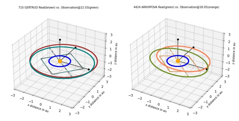
We computed orbital elements of our asteroids by using Find_Orb software depending on our observations’ right ascension and declination values obtained by using Astrometric. By our python code, we plot them as in the below figures together with their corresponding orbits retrieved from the ESA NEOCC asteroid database.
4. Estimating physical properties of the Asteroid
In addition to calculating the asteroid’s orbital parameters from its movement in front of the night sky it is possible to calculate an approximation of some of its physical properties. In such a manner many asteroids’ rotation periods are calculated from an analysis of their apparent magnitude - a value which is easily extractable from our own observations. In order to get results one observation would not suffice - to the contrary, many observations have to be done over a large timespan (months to years). This endeavour undertaken by many observatories worldwide leads to a light curve, displaying the asteroid’s change of magnitude over time. Since the vast majority of asteroids are not of spherical shape, its visible sunlight reflecting area changes periodically with its rotation. Thus the asteroid’s rotational period is equivalent to the period found in the created light curve.
Depending on the scrutiny regarding the observations and amount of collected data, it is possible to derive further information about the asteroid from the light curve such as a rough
estimate of the asteroid’s shape. In the case of binary systems, it is even achievable to calculate the asteroids’ mass from their perturbation on one another’s rotational period,
leading to their mass ratio, distances and binary periods.
Our observations are by far not enough to derive a usable light curve, but our magnitude data show a good fit to the rest of the observation.
5. Discussion on Unsuccessful Observations
For Group 1, we conducted several observations in the past few months tracing asteroids of Gertrud, Arkhipova and Helio. As permitted by the weather, and the condition of the observatory, several of them are unfortunately unsuccessful. Here we discuss possible reasons why these observations failed in tracing asteroids.
a) Observation of Gertrud on 11.06.2022
As the network in the observatory was broken on that day, we were not able to track asteroids via KStars (INDI) as usual. So in this case, we had to manually track the asteroids by typing RA and Dec. values. In order to gain the RA and Dec values as they were not included in the fits file due to the manual maneuver of the mount, a frame is uploaded to the Astrometry website to retrieve RA and Dec. values.
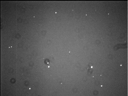
The main problem was that we used a low exposure of 90 sec, which was comparatively lower than the needed exposure to capture Gertrud.
For the processing process in Astrometrica, the images obtained didn’t show abundant stars (Figure. 6), which made the “Make data reduction” function unable to work. For this function, it needs more stars to be able to work properly.
b) Observation of Arkhipova on 11.06.2022
As we also observed Arkhipova on the same day as Gertrud, the same condition regarding manual tracking also applies to the observation of Gertrud. Besides, the telescope was
pointed to another direction, which resulted in an inaccurate heading.
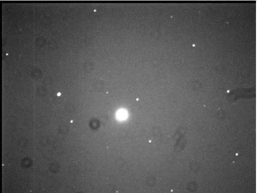
Despite a low exposure of 90 seconds, the star on the image is so bright (Figure. 7) that it disturbs the image and results in the failure in processing in astrometrica.
c)Observation of Gertrud on 18.06.2022
(Same reason as the observation conducted on 11.06.2022)
d)Observation of Gertrud and Helio on 25.06.2022
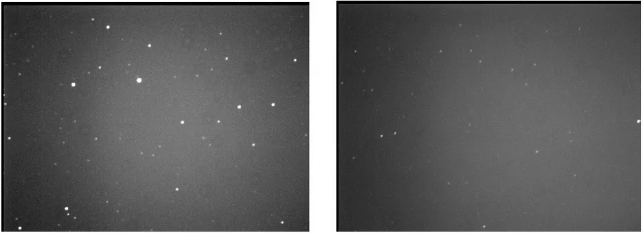
The weather condition was not ideal, as the weather became cloudy after the first trial image of Gertrud. Then the telescope was directed to the East where Helio was located (because it was cloudless at that moment). However, that area turned cloudy as well after the first shot.
The impact of clouds can be seen when the first and second set of images of Gertrud and Helio are compared. The image gets blurry and dim stars are not visible anymore (Figure. 8).
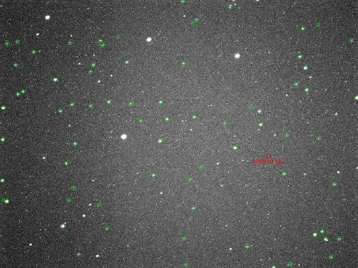
e)Observation of Helio on 24.07.2022
As the server of the observatory was still not working, we did the control of the mount manually. This time, the telescope was pointed to the correct RA and dec. and exposure of 150 sec. was used.
Though the images taken from the observation of Helio (Figure. 9) look promising for successful processing in Astrometrica, there exists one problem - although Astrometrica confirms that Helio is inside the frame after the tool of "Known Object Overlay", the asteroid itself is not visible in the frame. This is probably because the asteroid is much deviated from the MPC database. One of the alternatives for this situation is to use a telescope with less focal length, which is more suitable for this mission.
6. References
- https://minorplanetcenter.net/cgi-bin/checkmp.cgi
- http://www.astrometrica.at/
- Raab, Herbert. "Detecting and measuring faint point sources with a CCD." In Proceedings of Meeting on Asteroids and Comets in Europe (MACE), pp. 1-12. 2002.
- https://www.minorplanetcenter.net/iau/info/OpticalObs.html
- http://adams.dm.unipi.it/~orbmaint/orbfit/
- https://www.projectpluto.com/